Isogeny-based Cryptography
- Isognies
Isognies
(Warning: This is just a brief note, so it may contain some errors.)
Introduction to Isogenies
Let $E_1, E_2$ be the elliptic curves over a finite field $\mathbb{F}_q$. Here $q$ is some prime power. As far as we known, $(E_1,+)$ form a group under the addition of points and as $F_q$ is finite, so are these groups. So now we want to consider a map between these two elliptic curves:
What do we actually mean by this? To define such a map, we need to understand or provide an explicit formula describing the structure of these two curves. We also wonder what properties should this map have for it to “behave well” in both the geometric and algebraic sense?
- $\phi$ acts on points on the EC, which have an $x$ and a $y$ coordinate. So we can write $\phi = (\phi_1, \phi_2)$, which acts on a point $P = (x,y)$ on $E_1$ in the following way:
- We want this map to be rational. By this we mean that if $\phi = (\phi_1,\phi_2)$ then $\phi_1$ and $\phi_2$ are just algebraic fractions where the denominator and numerator are polynomials. For example
- We want $\phi$ to have this property, because it is a well known fact in maths that a rational map is either surjective or constant. Though this may not seem important, once we define a few more properties and start looking at isogenies, this becomes really useful.
- As both $E_1$ and $E_2$ form groups, ideally we would like $\phi$ to be a group homomorphism. Intuitively, this means that $\phi$ will preserver the group structure. Mathematically, if $+$ is the group operation on $E$, and $P,Q$ are two points on $E_1$ then:
Review:
Rational map A rational map from a variety $X$ to a variety $Y$ (over a field $K$) is a map that can be expressed using ratios of polynomials in the coordinates of $X$. Formally:
is a rational map if, for each coordinate function of $Y$, there exist a polynomial numerator and denominator in the coordinates of $X$ such that
for $i = 1,…, \dim Y$ and $f_i,g_i \in K[x_1,x_2,…,x_n]$
You can read more from here: https://en.wikipedia.org/wiki/Rational_mapping
For example: A rational map $\phi : E_1 \rightarrow E_2$ could be
Definition 1. A rational map $\phi: E_1 \rightarrow E_2$ is called an isogeny if $\phi(\mathcal{O}_1) = \mathcal{O}_2$ where $\mathcal{O}_i$ is the identity of the group $E_i$.
A famous example of an isogeny when we’re working over a finite field $\mathbb{F}_q$ is the Frobenius Map. If $P = (x,y)$, this map is given by
Rational functions
Let $\displaystyle E( K)$ be an elliptic curve with equation $\displaystyle f( X,Y) =0$. Take a polynomial $\displaystyle g( X,Y)$ and consider its behavior on the points of $\displaystyle E( K)$ only, ignoring its behaviour on all other values of $\displaystyle X$ and $\displaystyle Y$.
If $\displaystyle g=f$ then from our point of view, $\displaystyle g$ is the same as the zero function because $\displaystyle g( P) =0$ for any point $\displaystyle P$ on the curve. Then by Hilbert’s Nullstellensatz theorem, a polynomial $\displaystyle g$ is the zero function if and only if it is a multiple of $f$.
This leads us to define the ring of regular functions of $\displaystyle E$ to be
Its field of fractions $\displaystyle K[ E]$ is called the field of rational functions of $\displaystyle E$.
Note: There are two version of Hilbert’s Nullstellensatz theorem, you can look it up on any algebraic geometry textbook
Let $\displaystyle F$ be a algebraically closed field, $\displaystyle x^{d} =( x_{1} ,…,x_{d}) \in F^{d}$ and $\displaystyle P_{1} ,…,P_{m} \in F[ x]$ are polynomials in $\displaystyle d$ variables.
Weak nullstellensatz. Let $\displaystyle P_{1} ,…,P_{m} \in F[ x]$ be polynomials, here $\displaystyle F$ is a algebraically closed field. Then exactly one of the following statements hold:
-
The system of equations $\displaystyle P_{1}( x) =…=P_{m}( x) =0$ has a solution $\displaystyle x\in F^{d}$
-
There exist polynomials $\displaystyle Q_{1} ,…,Q_{m} \in F[ x]$ such that $\displaystyle Q_{1} P_{1} +…+Q_{m} P_{m} =1$.
Strong nullstellensatz. Same stament as above, but here we consider another polynomial $\displaystyle R\in F[ x]$. Then exactly one of the following statements hold:
-
The system of equations $\displaystyle P_{1}( x) =…=P_{m}( x) =0,R( x) \neq 0$ has a solution $\displaystyle x\in F^{d}$
-
There exist polynomials $\displaystyle Q_{1} ,…,Q_{m} \in F[ x]$ and a non negative integer $\displaystyle r$ such that $\displaystyle P_{1} Q_{1} +…+P_{m} Q_{m} =R^{r}$.
Endomorphisms
Definition: If $E_1 = E_2$ then $\phi$ is called an endomorphism. An endomorphism is an isomorphism if it is bijective. Review that $\phi$ is either the identity or surjective, so we only need to check if $\phi$ is injective.
An injective function is a function $f$ that map distinct elements of its domain to distinct elements of its codomain; that is, for $x1 \neq x2$ implies $f(x_1) \neq f(x_2)$.
The set of endomorphisms of an elliptic curve $E$ together with the zero map (the map that sends everything to zero) actually forms a ring under the operations of pointwise addition and multiplication given by composing the endomorphisms $(f \times g) = f(g(x)))$ .
A ring means that the addition and multiplication behave nicely and interact well with each other. I will write this down again for archival purpose:
Ring. A ring is an algebraic structure consisting of a set with two binary operations called addition and multiplication. Also:
- it is a group under the addition
- the multiplication is associative and has an identity
- multiplication is distributive with respect to addition
We denote this ring by $End(E)$. The zero map act as an additive identity and the identity map $id : P \rightarrow P$ is the multiplicative identity. For example we can consider the endomorphisms $f(P)=2P$ and $g(P)=3P$ for $P \in E$. Then we have their pointwise addition as follow:
j - invariant
Usually we write the Weierstrass equation for our elliptic curve using non-homogeneous coordinates $x=X/Z$, and $y=Y/Z$
and point $O=[0,1,0]$ out at infinity. If $a_1,…,a_6 \in K$ then $E$ is said to be defined over $K$. If $char(\overline{K})\neq 2$, then we can simplify the equation by completing the square. Thus the substitution
gives an equation of the form
where
We also define quantities
The quantity $\Delta$ is the discriminant of the Weierstrass equation, the quantity $j$ is the $j$ - invariant of the elliptic curve.
The $j$ - invariant help us to keep track the isomorphic class of an given elliptic curve. Two elliptic curves might have very different Weierstrass equation but if their $j$ - invariant are the same, they are isomorphic ( over the algebraic closure of $K$; that is, $\overline{K}$).
For Weierstrass equation $y^2=x^3+ax+b$ with char $\neq$ 2,3, the $j$ - invariant is equal to $j(E) = 1728 \times \frac{4a^3}{4a^3+27b^2}$
More precisely, we consider the equivalence classes of elliptic curves, where $E_1$ and $E_2$ are equivalent if and only if they are isomorphic.
Theorem Let $E$ and $E’$ be elliptic curves over $\mathbb{Q}$. The $E \cong E’$ over $\mathbb{C}$ if and only if $j(E) = j(E’)$. In general, given a field $K$ and elliptic curves $E,E’$ over $K$ then $E\cong E’$ over $\overline{K}$ if and only if $j(E) = j(E’)$.
Equality of $j$ - invariants does not guarantee an isomorphism over $\mathbb{F}_q$. Curves with same $j$ can be twists of each other.
Example: Consider the quadratic twists of a given curve. We will work with the elliptic curves $E: y^2=x^3+x$ over $\mathbb{F}_5$. The quadratic twists of $E$ is define as follow: here
Consider a quadratic nonresidue $d$ of $\mathbb{F}_5$. That is, choose an element $d$ such that $d \in \mathbb{F}_p$ but $\sqrt{d} \in \overline{\mathbb{F}_p}$ , i.e the algebraic closure of our field.
Then we can define another curve with the same $j$ - invariant as $E$:
And we have $ E’:y^2=x^3+2x$
We can calculate the $j$ - invariant by sagemath
sage: F = GF(5)
sage: E = EllipticCurve(F,[1,0])
sage: print(E)
Elliptic Curve defined by y^2 = x^3 + x over Finite Field of size 5
sage: E_ = EllipticCurve(F, [2,0])
sage: print(E.j_invariant())
3
sage: print(E_.j_invariant())
3
sage:
Degree and separability
We have the following definition: Degree of map: Let $\phi : E_1 \rightarrow E_2$ be a map of curves defined over $K$. If $\phi$ is constant, we define the degree of $\phi$ to be 0. Otherwise we say that $\phi$ is a finite map and we define its degree to be
We say that $\phi$ is separable, inseparable, or purely inseparable if the field extension $K(E_1)/\phi^*K(E_2)$ has the corresponding property, and we the separable and inseparable degrees of the extension by $\deg_s\phi$ and $\deg_i\phi$ .
Let make it more clear. We have known that every non-zero isogeny $\phi :E_1 \rightarrow E_2$ between elliptic curves of the form $y^2=f(x)$ can be written in the standard affine form
where $u \perp v$ and $s \perp t$ are pairs of relatively prime polynomials in $K[x]$ The degree of this map is actually equal to $\max \lbrace \deg p, \deg q \rbrace$ . The isogeny $\phi$ is separable if we have $(u/v)’ \neq 0$ where $(u/v)’$ denote the derivatives of rational function.
For example, consider the isogeny that map $P \rightarrow 2P$ as follow:
This is a map of degree 4 and is separable. So basically the degree of a non-zero separable isogeny is the number of elements in its kernel and it is also the degree of the isogeny as a rational map
For more details you should read this lecture notes. (i think i will skip this since the maths is too intense lol)
Another important key fact is that the finite subgroups $G\subset E_1$ are in one-to-one correspondence with the separable isogenies $\phi :E_1 \rightarrow E_2$, up to isomorphism of the codomain. That is
where $E_1/G$ is the quotient elliptic curve and $\ker(\phi) = G$.
Knowing the kernel, one can write down the isogeny explicitly base on the fact that each kernel uniquely define the map. We will later learn how to calculate this by using Velu’s formula
Isomorphisms are actually a special case of an isogeny where the kernel is trivial, in this case, the kernel is just ${\mathcal{O}}$
Isomorphisms vs isogenies
We know that if $\phi: E_1 \rightarrow E_2$ is an isomorphism then there is an inverse map $\phi^{-1}: E_2 \rightarrow E_1$ and their compose map gives us the identity map. Recall that an isogeny is a group homomorphism between two curves that map the identity on $E_1$ to the identity on $E_2$. So in general, there is no guarantee of invertibility because $\phi$ usually has a nontrivial kernel. However, every isogeny $\phi$ has a unique dual isogeny which we denote as $\hat{\phi}$ . Rather than composing to give the identity, if $\phi: E_1 \rightarrow E_2$ is an isogeny of degree $d$, then $\hat{\phi}$ is an isogeny of degree $d$ and the composition gives us $\phi \circ \hat{\phi} = [d]$ where $[d] : E_1 \rightarrow E_2$ is the multiplication by $d$ map.
Torsion Points
The group of all points $P$ on $E_1$ such that $[d]P = \mathcal{O}$ is denoted by $E_1[d]$ and are called the $d$-torsion points. In other words, these are the points that are in the kernel of the multiplication by $d$ map.
Theorem. Let $\displaystyle E/k$ be an elliptic curve and $\displaystyle d$ a non zero integer. If $\displaystyle char( k) =p >0$, factor $\displaystyle d$ as $\displaystyle m\times p^{r}$ with $\displaystyle m\notin p\mathbb{Z}$, otherwise, let $\displaystyle m=d$. Then as groups:
In particular $\displaystyle E[ p] \cong \mathbb{Z} /p$ or $\displaystyle E[ p] \cong {0}$ and if $\displaystyle char( k)\not{\mid } d$ then $\displaystyle E[ d] \cong \mathbb{Z} /d\times \mathbb{Z} /d$.
This come from the fact that every finitely generated abelian groups classify as products of cyclic groups.
Furthermore we have #$E[d] = d^2$
You can also read this notes for further research https://www.math.uchicago.edu/~may/VIGRE/VIGRE2008/REUPapers/Travis.pdf
For an elliptic curve over $\mathbb{C}$, it can be written as a torus
The map $[d]$ corresponds to scaling by $d$ which gives us
The kernel is actually the lattice points $\displaystyle \frac{1}{d} \Lambda /\Lambda$ which forms a grid of size $\displaystyle d^{2}$. That’s why we always get $d^2$ torsion points.
Divisor and division polynomials
The divisor of a curve $\displaystyle E$ denote by $\displaystyle div( E)$ is the free abelian group generated by the points of $\displaystyle E$. Thus a divisor $\displaystyle D\in div( E)$ is a formal sum:
where $\displaystyle n_{p} \in \mathbb{Z}$ and $\displaystyle n_{p} =0$ for all but finitely many $\displaystyle P\in E$. The degree of $\displaystyle D$ is defined by
For example we have $\displaystyle D=2[ P] -[ Q] +[ R]$ then the degree of $\displaystyle D$ will be $\displaystyle 2-1+1=2$.
For more detail see here: https://crypto.stanford.edu/pbc/notes/elliptic/funcfield.html
Division polynomials are built from divisors of multiplication maps, and they encode torsion points. They also provide a way to calculate multiples of points on elliptic curves.
Definition (see also exercise 3.7 in silverman boook for a more generic formula)
Let $\displaystyle E:y^{2} =x^{3} +Ax+B$ be an elliptic curve over some field $K$ . The set of division polynomials is a sequence of polynomials in $\displaystyle \mathbb{Z}[ x,y,A,B]$ that is recursively defined by
and then inductively by the formulas
$\displaystyle \psi _{2m}$ is also a polynomial for all $\displaystyle m\geqslant 1$, and then define further polynomials $\displaystyle \phi _{m}$ and $\displaystyle \omega _{m}$ by
Given a point $\displaystyle P=( x_{p} ,y_{p})$ on the elliptic curve $\displaystyle E:y^{2} =x^{3} +Ax+B$ over some field $\displaystyle K$, we can express the coordinates for the $\displaystyle n^{th}$ multiplpe of $\displaystyle P$ in terms of division polynomials:
In sage, we can use E.division_polynomial(k) to call the $k^{th}$ division polynomial
sage: E = EllipticCurve(GF(101),[2,3])
sage: print(E.division_polynomial(5))
5*x^12 + 23*x^10 + 29*x^9 + 85*x^8 + 26*x^7 + 86*x^6 + 31*x^5 + 2*x^4 + 27*x^3 + 62*x^2 + 30*x + 52
Read more: Docs
Another method to call is E.multiplication_by_m(k).
Practice
https://cryptohack.org/challenges/isogenies/
Image Point Arithmetic
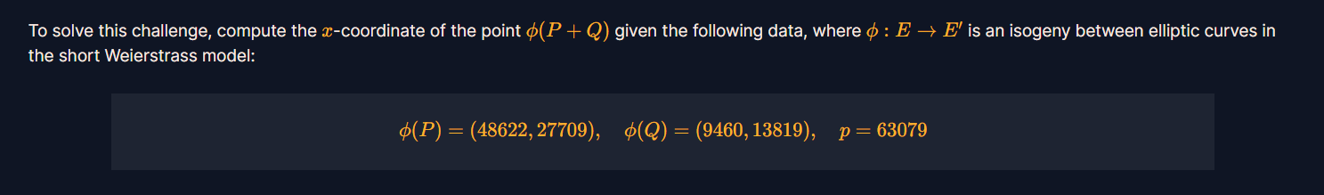
For this challenge we can applied the property $\phi(P)+\phi(Q) = \phi(P+Q)$ since the isomorphism preserves the group structure
from sage.all import *
p=63079
Px = 48622
Py = 27709
Qx = 9460
Qy = 13819
a = (((Py**2-Qy**2)-(Px**3-Qx**3))*pow(Px-Qx,-1,p)) % p
b = (Py**2  - Px**3 - a*Px )% p
E = EllipticCurve(GF(p), [a,b])
P = E(Px,Py)
Q = E(Qx,Qy)
print(P+Q)
Montgomery Curves
Here we are given an elliptic curve over $p=1912812599$,
There are three solutions to this problem.
The first one we can simply use the function E.montgomery_model(). This should be available in the newest version of sagemath
The second solution can be explained by following the approach in https://eprint.iacr.org/2017/212.pdf. ince the two curves are related by a degree-one isogeny, their $j$-invariants are equal. For Montgomery curves, the $j$-invariant is calculated as follows:
from sage.all import *
p = 1912812599
E = EllipticCurve(GF(p),[312589632,654443578])
j = E.j_invariant()
P = PolynomialRing(GF(p),'A')
A = P.gen()
f = 256*(A**2-3)**3-j*(A**2-4)
roots = f.roots(multiplicities = False)
for r in roots:
    r_ = int(r)
    EM = EllipticCurve(GF(p),[0,r_,0,1,0])
    if EM.j_invariant() == j:
        print(r_)
The third solution relies on the two-torsion trick. By mapping a 2-torsion point from the short Weierstrass model to $(0:0:1)$ on the Montgomery model, we can derive the corresponding Montgomery coefficient.
So indeed, the 2-torsion point of $E$ correspond to another 2-torsion point of $E’$. We can pick a 2-torsion point of $E$, for example $(r,0)$ and make the translation $x \rightarrow X + r$ that send our original curve to its Montgomery form
This guarantees that the chosen torsion point $(r,0)$ in Weierstrass form becomes $(0,0)$ in the new coordinate system.
DLOG on the Surface
Source code:
import os
from Crypto.Cipher import AES
from Crypto.Hash import SHA256
from Crypto.Util.Padding import pad

proof.all(False)

FLAG = b"crypto{?????????????????????????????????????????????????????????????}"

p = 2**127 - 1
F.<i> = GF(p^2, modulus=[1,0,1])
E = EllipticCurve(F, [1,0])
P, Q = E.gens()

a = randint(0, p) | 1
b = randint(0, p) | 1
c = randint(0, p) | 1
d = randint(0, p) | 1

R = a*P + b*Q
S = c*P + d*Q

def encrypt_flag(a, b, c, d):
    data_abcd = str(a) + str(b) + str(c) + str(d)
    key = SHA256.new(data=data_abcd.encode()).digest()[:128]
    iv = os.urandom(16)
    cipher = AES.new(key, AES.MODE_CBC, iv)
    ct = cipher.encrypt(pad(FLAG, 16))

    return iv.hex(), ct.hex()

iv, ct = encrypt_flag(a, b, c, d)

print(f"{P = }")
print(f"{Q = }")
print(f"{R = }")
print(f"{S = }")
print()
print(f"{iv = }")
print(f"{ct = }")
In this challenge, we are given four points $P,Q,R,S$ of elliptic curve $E$. The curve is described as follow:
p = 2**127 - 1
F.<i> = GF(p^2, modulus=[1,0,1])
E = EllipticCurve(F, [1,0])
P, Q = E.gens()
Our base field is $\mathbb{F}_{p^2} \cong \mathbb{F}_p[X]/(X^2+1)$ and we choose $\displaystyle p\equiv 3\bmod 4$ so that the polynomial $\displaystyle X^{2} +1$ has no root and is irreducible.
Moreover, there are relations between our given points:
Our goal is to find $\displaystyle a,b,c,d$ and recover the secret key. Because we are working on supersingular elliptic curves over $\displaystyle \mathbb{F}_{p^{2}}$, the abelian group of points on the curve is isomorphic to $\displaystyle \mathbb{Z} /( p+1) \times \mathbb{Z} /( p+1)$
Every point in $\displaystyle E(\mathbb{F}_{p^{2}})$ an be expressed as a combination of two independent generators, in our case, they are $\displaystyle P$ and $\displaystyle Q$.
For the torsion subgroup $\displaystyle E[ n]$, if $\displaystyle \gcd( n,p) =1$. For the torsion subgroup $\displaystyle E[ n]$, if $\displaystyle \gcd( n,p) =1$ then $\displaystyle E[ n] \cong \mathbb{Z} /n\times \mathbb{Z} /n$.
To solve this challenge I will use the Weil’s pairing. For more details, one should read the section 1.7 and 1.9 from this notes https://yx7.cc/docs/misc/isog_bristol_notes.pdf
The order of our curve is $(p+1)^2$ and this is also the order of $P,Q,R,S$. We will have
Since the order is $2^{127}$, solving DLP should be easy. See also the MOV attack / Weil pairing explanation: https://risencrypto.github.io/WeilMOV/
We will do the same for $b,c,d$. Note that $e(P,Q)e(Q,P)=1$. Solve script:
from sage.all import *
from Crypto.Cipher import AES
from Crypto.Hash import SHA256
p = 2**127 - 1
F = GF(p**2, name='i', modulus=[1,0,1])
i = F.gen()
E = EllipticCurve(F,[1,0])


P = E(24722427318870186874942502106037863239*i + 62223422355562631021732597235582046928 , 66881667812593541117238448140445071224*i + 149178354082347398743922440593055790802)
Q = E(136066972787979381470429160016223396048*i + 52082760150043245190232762320312239515 , 37290474751398918861353632929218878189*i + 89777436105166947842660822806860901885)
R = E(115434063687215369570994517493754451626*i + 158874018596958922133589852067300239562 , 62259011436032820287439957155108559928*i + 81253318200557694469168638082106161224)
S = E(42595488035799156418773068781330714859*i + 113049342376647649006990912915011269440 , 25404988689109287499485677343768857329*i + 125117346805247292256813555413193592812)

iv = '6f5a901b9dc00aded4add3791812883b'
ct = '56ecb68a90cad9787a24a4511720d40d625901577f6d0f1eef9fc34cf042709110cdc061fff91e934877674a30ed911283b83927dbcc270ae358d6b1fe2d5bed18ce1b02d8805de55e5b36deb0d28883'
n = P.order()
base = P.weil_pairing(Q,n)
a = discrete_log(R.weil_pairing(Q,n),base,n)
b = (-discrete_log(R.weil_pairing(P,n),base,n)) % n
c = discrete_log(S.weil_pairing(Q, n),base,n)
d = (-discrete_log(S.weil_pairing(P, n),base,n)) % n
key = SHA256.new(f'{a}{b}{c}{d}'.encode()).digest()[:128]
iv = bytes.fromhex('6f5a901b9dc00aded4add3791812883b')
ct = bytes.fromhex('56ecb68a90cad9787a24a4511720d40d625901577f6d0f1eef9fc34cf042709110cdc061fff91e934877674a30ed911283b83927dbcc270ae358d6b1fe2d5bed18ce1b02d8805de55e5b36deb0d28883')
print(AES.new(key, AES.MODE_CBC, iv).decrypt(ct).strip())
You can check whether this curve is supersingular or not by using the function: E.trace_of_frobenius() % p == 0
Note: Currently im using SageMath version 10.6 so this function should be working. Lets try it.
p = 2**127 - 1
F = GF(p**2, name='i', modulus=[1,0,1])
i = F.gen()
E = EllipticCurve(F,[1,0])


P = E(24722427318870186874942502106037863239*i + 62223422355562631021732597235582046928 , 66881667812593541117238448140445071224*i + 149178354082347398743922440593055790802)
Q = E(136066972787979381470429160016223396048*i + 52082760150043245190232762320312239515 , 37290474751398918861353632929218878189*i + 89777436105166947842660822806860901885)
R = E(115434063687215369570994517493754451626*i + 158874018596958922133589852067300239562 , 62259011436032820287439957155108559928*i + 81253318200557694469168638082106161224)
S = E(42595488035799156418773068781330714859*i + 113049342376647649006990912915011269440 , 25404988689109287499485677343768857329*i + 125117346805247292256813555413193592812)
n = P.order()
base = P.weil_pairing(Q,n)
a = discrete_log(R.weil_pairing(Q,n),base,n)
b = (-discrete_log(R.weil_pairing(P,n),base,n)) % n
a_,b_ = E.abelian_group().discrete_log(R,[P,Q])
print(a,b, '\n')
print(a_ % n ,b_ % n ,'\n')
One should also including two generators [P,Q]. Without it the result will be different.
Docs
sage: x = polygen(ZZ, 'x')
sage: F.<t> = GF(1009**2, modulus=x**2+11); E = EllipticCurve(j=F(940))
sage: P, Q = E(900*t + 228, 974*t + 185), E(1007*t + 214, 865*t + 802)
sage: E.abelian_group().discrete_log(123 * P + 777 * Q, [P, Q])
(123, 777)
sage:
SIDH
Now , lets talk about SIDH and Velu’s formula. There are some prequisite topics that need to be mention again.
Supersingular curve
Theorem. Let $K$ be a field of characteristic $p$, and let $E/K$ be an elliptic curve. For each integer $r \geq 1$, let
be the $\displaystyle p^{r}$ - power frobenius map and its dual.
Then the following are equivalent: i/ $\displaystyle E\left[ p^{r}\right] =0$ for one(all) $\displaystyle r\geqslant 1$
ii/ $\displaystyle \hat{\phi }_{r}$ is purely inseparable for one(all) $\displaystyle r\geqslant 1$
iii/ The map $\displaystyle [ p] :E\rightarrow E$ is purely inseparable and $\displaystyle j( E) \in \mathbb{F}_{p^{2}}$.
iv/ $\displaystyle End( E)$ is an order in a quaternion algebra
If E has the properties given above, then we say that $E$ is supersingular or that $E$ has hasse invariant 0
Some deeper properties are unnecessary to mention here, however it is important to note that supersingular curves are all define over $\mathbb{F}_{p^2}$
SIDH Scheme
At first, I was reading from this paper: https://eprint.iacr.org/2011/506.pdf
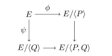
The SIDH Scheme revolve around the following commutative diagram
First, fix the finite field
where
In the original SIDH paper, we choose $(l_A,l_B)=(2,3)$ and an integer $f$ is chosen such that $p$ is a prime number.
We want the same security level for Bob and Alice , then we set $l_{A}^{e_A} \approx l_{B}^{e_B}=2^{O(\lambda)}$, where $\lambda$ is a security parameter.
Then we choose a random supersingular curve $E$ over $\mathbb{F}_q$ such that
We use isogenies, $\phi_A,\phi_B$ with kernels of order $l_{A}^{e_A},l_{B}^{e_B}$, respectively and the following commutative diagram for the SIDH key exchange between Alice and Bob
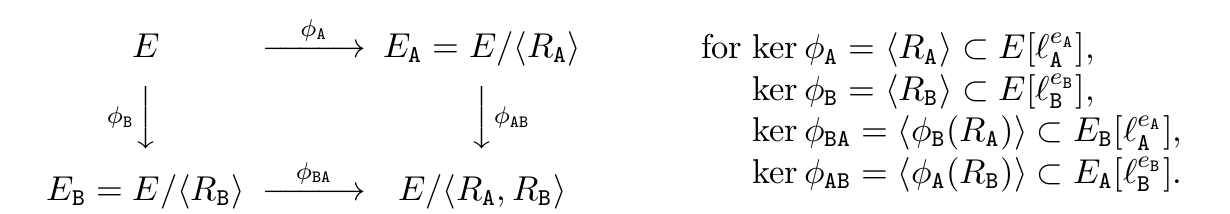
From the diagram we can see: We first start with an supersingular curve ${\displaystyle E=E_{0}}$ over ${\displaystyle \mathbb{F}_{p^{2}}}$.
Alice then choose a subgroup ${\displaystyle \langle R_{A} \rangle \subseteq E\left[ l_{A}^{e_{A}}\right]}$, Bob also choose a subgroup ${\displaystyle \langle R_{B} \rangle =E\left[ l_{B}^{e_{B}}\right]}$.
The two isogenies are $\displaystyle \phi_{A} :E\rightarrow E_{A}$ and $\displaystyle \phi_{B} :E\rightarrow E_{B}$.
Both paths end up at the same final curve ${\displaystyle E_{AB} =E_{BA} =E/\langle R_{A} ,R_{B} \rangle }$
The torsion subgroup ${\displaystyle E\left[ l_{A}^{e_{A}}\right]}$ will have two torsion bases ${\displaystyle P_{A} ,Q_{A}}$. Same for ${\displaystyle P_{B} ,Q_{B}}$.
We define the generators as ${\displaystyle pk^{\text{sidh}} =(g=(E;P_{A} ,Q_{A} ,P_{B} ,Q_{B} )),\ e\ =\ (l_{A} ,l_{B} ,e_{A} ,e_{B} ))\leftarrow Gen^{\text{sidh}}\left( 1^{\lambda }\right)}$
Implement: You can also see this talk by Lorenz Panny
#public
lA, eA, lB, eB = 2, 91, 3, 57
p = lA^eA * lB ^ eB - 1
F.<i> = GF(p^2, modulus=x^2+1)
E0 = EllipticCurve(F, [1, 0])
PA, QA = (lB^eB * G for G in E0.gens())
PB, QB = (lA^eA * G for G in E0.gens())

#Alice
privA = randrange(lA^eA)
KA = PA + privA*QA
phiA = E0.isogeny(KA, algorithm="factored")
pubA = (phiA.codomain(), phiA(PB), phiA(QB))

#Bob
privB = randrange(lB^eB)
KB = PB + privB*QB
phiB = E0.isogeny(KB, algorithm="factored")
pubB = (phiB.codomain(), phiB(PA), phiB(QA))

#Alice
LA = pubB[1] + privA*pubB[2]
psiA = pubB[0].isogeny(LA, algorithm="factored")
sharedA = psiA.codomain()

#Bob
LB = pubA[1] + privB*pubA[2]
psiB = pubA[0].isogeny(LB, algorithm="factored")
sharedB = psiB.codomain()

assert sharedA == sharedB
print(sharedA)
Velu’s formula
We have seen that abstractly, isogenies are determined by their kernels. There are some algorithms to compute separable isogenies from their kernel given the following results: Let $\displaystyle E/k$ be an elliptic curve in Weierstrass form, and $\displaystyle G$ a finite subgroup of $\displaystyle E(\overline{k})$. Let $\displaystyle G_{\neq 0}$ denote the set of nonzero points in $\displaystyle G$, which are affine points $\displaystyle Q=( x_{Q} ,y_{Q})$.
For all affine points $\displaystyle P=( x_{P} ,y_{P})$ in $\displaystyle E(\overline{k})$ and not in $\displaystyle G$ define:
Here $\displaystyle x_{P} ,y_{P}$ are variables, $\displaystyle x_{Q} ,y_{Q}$ are elements of $\displaystyle \overline{k}$ and $\displaystyle x_{P+Q} ,y_{P+Q}$ are rational functions of $\displaystyle x_{P} ,y_{P}$ giving coordinates of $\displaystyle P+Q$ in term of $\displaystyle x_{P}$ and $\displaystyle y_{P}$.
For $\displaystyle P\notin G$ we have $\displaystyle \alpha ( P) =\alpha ( P+Q)$ if and only if $\displaystyle Q\in G$ so $\displaystyle \ker \alpha =G$
In general, these formulas are just rational functions of the output mentioned above and the degrees of these functions are the same size as the size of the kernel $G$.
We can see that to evalute Velu’s formula takes $O(|G|)$ operation and the cost is exponential in $\log(\deg(\phi))$ where $\phi$ is the map that map $E \rightarrow E/G$ and $P \rightarrow \alpha(P)$
In practice, we will use the two following theorems:
Theorem 1. Let $\displaystyle E:y^{2} =x^{3} +Ax+B$ be an elliptic curve over $\displaystyle k$ and let $\displaystyle x_{0} \in \overline{k}$ be a root of $\displaystyle x^{3} +Ax+B$. Define $\displaystyle t:=3x_{0}^{2} +A$ and $\displaystyle w:=x_{0} t$. The rational map
is a separable isogeny from $\displaystyle E$ to $\displaystyle E’:y^{2} =x^{3} +A’x+B’$ where $\displaystyle A’:=A-5t$ and $\displaystyle B’:=B-7w$. The kernel of $\displaystyle \alpha$ is the group of order 2 generated by $\displaystyle ( x_{0} ,0)$. center
Theorem 2. Let $\displaystyle E:y^{2} =x^{3} +Ax+B$ be an elliptic curve over $\displaystyle k$ and let $\displaystyle G$ be a finite subgroup of $\displaystyle E(\overline{k})$ of odd order. For each non zero $\displaystyle Q=( x_{Q} ,y_{Q})$ in $\displaystyle G$ define
The rational map center
is a separable isogeny from $\displaystyle E$ to $\displaystyle E’:y^{2} =x^{3} +A’x+B’$ where $\displaystyle A’:=A-5t$ and $\displaystyle B’=B-7w$ with $\displaystyle \ker \alpha =G$.
Breaking SIDH
Coming soon …